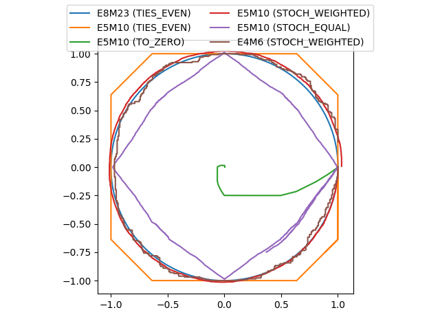
Floating-point ODE solver

This illustrates the effect of solving an ODE with forward Euler using different floating-point formats and different quantization schemes.

The ODE in question is

\[ \begin{align}\begin{aligned}u'(t) = v(t), \quad u(0) = 1,\\v'(t) = -u(t), \quad v(0) = 0,\end{aligned}\end{align} \]

and the solution is the unit circle in the (u, v) plane.

(Example was inspired from M. Croci, M. Fasi, N. J Higham, T. Mary, M. Mikaitis. “Stochastic Rounding: Implementation, Error Analysis, and Applications”, in Royal Society Open Science, 2022.)

import math

import matplotlib.pyplot as plt

import apytypes as apy


def solve_ode(exp_bits, man_bits, bias, iterations=2**14):
    h = 2 * math.pi / iterations
    ode = apy.fp([[0, h], [-h, 0]], exp_bits, man_bits, bias)
    current_value = apy.fp([1, 0], exp_bits, man_bits, bias)
    results = apy.zeros(
        (iterations + 1, 2), exp_bits=exp_bits, man_bits=man_bits, bias=bias
    )

    results[0, :] = current_value
    for i in range(iterations):
        current_value += ode @ current_value
        results[i + 1, :] = current_value
    return results


fig, ax = plt.subplots()

# Floating-point configurations: (exp_bits, man_bits, bias, quantization)
# Note: when the bias is set to None, it defaults to an IEEE-like bias
fp_formats = [
    (8, 23, None, "TIES_EVEN"),
    (5, 10, None, "TIES_EVEN"),
    (5, 10, None, "TO_ZERO"),
    (5, 10, None, "STOCH_WEIGHTED"),
    (5, 10, None, "STOCH_EQUAL"),
    (4, 6, 11, "STOCH_WEIGHTED"),
]

for exp_bits, man_bits, bias, mode in fp_formats:
    with apy.APyFloatQuantizationContext(
        eval(f"apy.QuantizationMode.{mode}"), quantization_seed=12
    ):
        results = solve_ode(exp_bits, man_bits, bias)
    ax.plot(results[:, 0], results[:, 1], label=f"E{exp_bits}M{man_bits} ({mode})")

ax.set_aspect("equal")
fig.legend(ncols=2, loc="upper center")
plt.show()